Thoughts on the nonlinear homogenization of dual phase, open cell meta materials, with a simple analytic example

October 21, 2023

Introduction

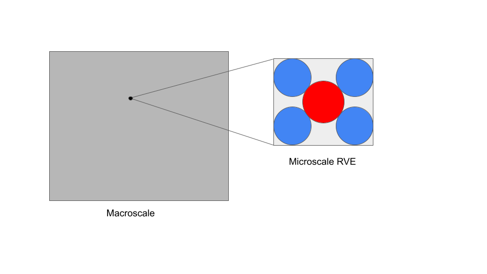
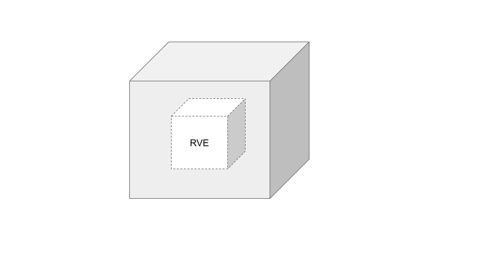
The goal of micro-structure homogenization is to effectively capture the macroscopic properties of a material based on the materials and geometry that exist on the micro-scale. To do this, one can make the assumption that each macro-scale material point is represented by a micro-scale representative volume element (RVE). Then, the deformation gradient at the macro-scale would be applied as a constant to the entire boundary of the micro-scale RVE, implying that the deformation at the entire RVE boundary is known and linear. If a material is periodic, the prescribed boundary condition characterization can be made more precise, but for now we will assume the constant deformation gradient boundary condition. It should be noted that homogenization could be carried out again to the nano scale all the way to individual atoms, but, assuming we have done our job well as continuum mechanicians, we should be able to get away with only looking at the micro-scale if we know constitutive relationships for the materials present there.

Currently, I am working on a project where we must derive a transversely isotropic macroscale strain energy function from a microscale RVE. The RVE in question is two phases: air and a neo-hookean polymer. In characterizing the finite deformation mechanical behavior of a dual phase open cell meta material where the second phase is air, we would then need only the strain energy function of the solid phase as we can assume air has zero strain energy. Any attempt to analytically characterize macro scale behavior via the micro structure would be completely unfeasible, so we are using finite element simulations to recreate the seven or so tests necessary to completely characterize transverse isotropic behavior. In this process, it became necessary to understand how to measure stress and deformation at the macroscale based on deformation at the microscale.

Luckily, the proof that the macro-scale deformation gradient is equal to the volume average (with respect to the reference configuration) of the deformation gradient given the boundary condition described above is fairly straight forward. In a course I have been studying on micro mechanics and homogenization[1], a similar idea for the stress was communicated rather ineffectively: for quasi-convex strain energy functions, the macro-scale first piola-kirchoff stress of a material is equal to the volume average (with respect to the reference configuration) of the micro-scale stress over the RVE. Since I do not believe this fact was emphasized enough for how non-trivial the proof is, I will do all the necessary steps here.

Theoretical formulation

Recall now that the macro-scale deformation gradient is applied as a constant tensor to the entire RVE outer surface. Therefore, deformation at any point on the surface of the RVE is linear and of the form u=Fx, where F is the macro-scale deformation gradient, x is the boundary point in the reference configuration, and u is the deformed boundary point. Note also that from this point on, "average" refers to the volume average of a quantity with respect to the reference configuration, and is represented symbolically by <>.

Claim: The macro-scale deformation gradient is equal to the average deformation gradient over the RVE.

Proof:

\[ \langle \mathbf{F} \rangle = \frac{1}{V} \int \mathbf{F} \, dV = \frac{1}{V} \oint \mathbf{u} \cdot \mathbf{N} \, dS = \frac{\overline{\mathbf{F}}}{V} \oint \mathbf{x} \cdot \mathbf{N} \, dS = \frac{\overline{\mathbf{F}}}{V} \int \frac{\partial \mathbf{x}}{\partial \mathbf{x}} \, dV = \overline{\mathbf{F}} \]

where divergence theorem is used, N is the normal vector in the reference configuration, and V is the referential volume.

Now, we seek to establish a similar relationship for the stress. Assuming we know each material's strain energy density per reference volume, it should be obvious that the macro-scale strain energy density, H, is the average strain energy density over the entire RVE:

\[ H(\overline{\mathbf{F}}) = \frac{1}{V} \int W(\mathbf{F}) \, dV \]

Where clearly F is a function of F. Now, naively, if we wanted to know the first piola-kirchoff stress at the macroscale, we world take a derivative of both sides to find

\[ \frac{\partial H}{\partial \overline{\mathbf{F}}}(\overline{\mathbf{F}}) = \frac{1}{V} \int \frac{\partial W}{\partial \mathbf{F}} : \frac{\partial \mathbf{F}}{\partial \overline{\mathbf{F}}}(\mathbf{F}) \, dV \]

where : denotes double contraction of tensors. This alone does not reveal much about the macro-scale stress. However, since equilibrium states are energy minimizers and the microscale strain energies are assumed quasiconvex, we can say more. Indeed, we can say that F minimizes the functional form H. So, if we instead represent F as F=F+ΔF, where ΔF is the deviation of the deformation gradient from the average on the interior of the RVE, we see that

\[ \frac{\partial H}{\partial \overline{\mathbf{F}}} : \delta \overline{\mathbf{F}} = \frac{1}{V} \int \frac{\partial W}{\partial \mathbf{F}} \left( \mathbf{1} + \frac{\partial \Delta \mathbf{F}}{\partial \overline{\mathbf{F}}} \right) : \delta \overline{\mathbf{F}} = \frac{1}{V} \int \left( \frac{\partial W}{\partial \mathbf{F}} : \delta \overline{\mathbf{F}} + \frac{\partial W}{\partial \mathbf{F}} : \frac{\partial \Delta \mathbf{F}}{\partial \overline{\mathbf{F}}} : \delta \overline{\mathbf{F}} \right) dV = 0 \]

When evaluated at the actual deformation gradient \( \overline{\mathbf{F}} \). Since this integral is taken over the whole RVE and it is assumed that there is no body force or traction, we know from the principal of virtual work that the integral of \( \frac{\partial W}{\partial \mathbf{F}} : \delta \overline{\mathbf{F}} \) is zero. Since \( \delta \overline{\mathbf{F}} \) is essentially arbitrary (it need only be an admissible deformation gradient), it stands to reason that \( \frac{\partial W}{\partial \mathbf{F}} : \frac{\partial \Delta \mathbf{F}}{\partial \overline{\mathbf{F}}} = 0 \). Therefore, we can then see from the previous expression for the derivative of the macro energy and our alternative expression for \( \mathbf{F} \) that

\[ \frac{\partial H}{\partial \overline{\mathbf{F}}}(\overline{\mathbf{F}}) = \overline{\mathbf{P}} = \frac{1}{V}\int \frac{\partial W}{\partial \mathbf{F}}(\mathbf{F})dV = \langle \mathbf{P} \rangle \]

Therefore, the (PK1) macro-stress is equal to the average PK1 micro-stress. Hence, in homogenization, to understand the stress displacement response of the macro-structure, one only needs to evaluate the average stress of the RVE subject to a homogeneous deformation along the boundary. Taking this further, one can actually determine macro-scale second derivatives of the strain energy to understand anisotropy, but if this is known a priori as it is for my current project, this step is not necessary. Instead, the derivation of this fourth order tensor is left to the reader (hint: take a second variation).

While one can carry out real or simulated experimental testing to fit an actual strain energy given the above insights, the problem of determining the macro scale strain energy analytically would require knowing F as an explicit function of a general F, which for most geometries is a completely unfeasible task. However, for a simple RVE and strain energy, the macro-scale strain energy function can be solved analytically.

Example of an analytical solution to a homogenization problem

Suppose a hollow cube (with cubic inclusion of air) of side length L and thickness t is made of an incompressible Varga material. Denote the porosity, or volume of voids, for the material by ε. Now, one might immediately question whether or not the macro-scale material is also incompressible, which would be necessary in analyzing what sort of gradients can be applied to the RVE boundary. This question is actually answered simply; indeed, if V denotes the reference volume of air and v denotes the current volume of air, then

\[ \begin{align*} V &= \int dV \\ &= \int \text{Div} \left( \boldsymbol{E_1} \otimes \boldsymbol{E_1} \right) \boldsymbol{X} \, dV \\ &= \oint \left( \boldsymbol{E_1} \otimes \boldsymbol{E_1} \right) \boldsymbol{X} \cdot \boldsymbol{N} \, dA \\ &= \oint \left( \boldsymbol{E_1} \otimes \boldsymbol{E_1} \right) \boldsymbol{X} \cdot \boldsymbol{F}^{T} \boldsymbol{n} \, da \\ &= \oint \boldsymbol{F}\left( \boldsymbol{E_1} \otimes \boldsymbol{E_1} \right) \boldsymbol{X} \cdot \boldsymbol{n} \, da \\ &= \int \text{div} \left( \boldsymbol{F}\left( \boldsymbol{E_1} \otimes \boldsymbol{E_1} \right) \boldsymbol{X} \right) \, dv \\ &= \int \text{Div} \left( \left( \boldsymbol{E_1} \otimes \boldsymbol{E_1} \right) \boldsymbol{X} \right) \, dv = \int dv = v \end{align*} \]

where the identity \( \text{div}(\mathbf{F}\mathbf{v})=\text{Div}(\mathbf{v}) \) for any \( \mathbf{v} \) is easily proven[3], and the divergence theorem, Nanson's formula, and the incompressibility of the solid is used liberally. Then, the initial and final volume of the air is always the same, so it can be assumed that the whole macro-material is incompressible. Thus, we should not have any problem characterizing the macro-structure behavior restricted to boundary gradients of determinant 1. Of course, it might be more accurate to assign a periodic boundary as opposed to a homogeneous one, but to simplify the analysis we maintain the homogeneous assumption. We make a further assumption: for homogeneous, linear boundary deformations, one would expect the shape of the inner cube to be an affine transformation of the outer cube. That is to say, the shape of the inside cube is the exact same as that of the outside cube. We can further assume that the shape would not be rotated as again, all boundary deformation is linear. Then, it would have to be the case that at an inner corner of the cube, the deformed basis vectors are parallel to the deformed basis vectors at the outer corner of the cube. This would imply that the deformation gradient of the inner cube is exactly the same as that of the outer cube, as they could only differ by multiplication by a scalar. This is not possible due to incompressibility, so the deformation gradient must be constant on this surface also. Since the air is homogeneous and has a constant boundary deformation gradient, we can assume that the air has an average deformation gradient equal to \( \mathbf{\overline{F}} \).

Now, the incompressible form of the Varga strain energy[2] is

\[ W(\mathbf{F}) = 2\mu(i_{1}-3) \]

where \( i_1 \) is the first invariant of \( \mathbf{\overline{F}} \). We can see that, if we can find the integral (with respect to the reference configuration of the solid) of only \( i_1 \) for a given \( \mathbf{\overline{F}} \), then we can derive explicitly the macro scale strain energy. This proves to be easy, given all the legwork we have already put in above:

\[ \begin{align} \int i_1dV_s & = \int \mathbf{F}:\mathbf{1}dV \\ & = \int \mathbf{F}:\mathbf{1}dV_S \\ & = \oint \mathbf{u}\cdot\mathbf{n}dA_S \\ & = \overline{F}_{ij}\oint x_jn_idS \\ & = \overline{F}_{ij}\int x_{j,i}dV \\ & = \mathbf{\overline{F}}:\mathbf{1}V_s \\ & = \overline{i_1}V_s \end{align} \]

So, from the equation for the macro-scale strain energy and the fact that the strain energy of the air is 0, the macro-scale strain energy is then

\[ \begin{align} H(\mathbf{\overline{F}}) & = \frac{2\mu V_s}{V}(\overline{i_1}-3) \\ & = 2\mu(1-\epsilon)(\overline{i_1}-3) \end{align} \]

Indicating, as one would expect, that the macro-scale stress of a cellular material is a function of both the deformation gradient and the porosity. This actually allows for one to incorporate a heterogeneous porosity distribution over the material, if one assumes that RVEs in different locations have different solid volume fractions. In fact, to aid in the accuracy of this solution, one is encouraged to apply a heterogeneous porosity distribution, as sufficient heterogeneity would imply that the material is not periodic. Further, notice how the ease of analysis relayed on the simplicity of the strain energy relationship and the assumptions possible given the geometry. One is rarely so fortunate.

For the complex geometry and strain energy I investigate in my current project, obtaining an analytical solution is obviously not feasible. However in better understanding the problem as it related to that project, I became curious about classes of problems where analytical solutions were possible. The concept of analytically determining these macro-scale strain energy functions remains intriguing, even if unimportant in the grand scheme of things.

References:

1. Shaofan Li, Gang Want, Introduction to Micromechanics and Nanomechanics, 2017
2. David J. Steigmann, Finite Elasticity Theory, 2017
3. Panayiotis Papadopoulos, ME 185: Introduction to Continuum Mechanics, 2020

-TJC